Income and Substitution Effects
Page Overview | Income and Substitution Effects | Female vs Male Behavior in the Labor Market | Opportunity Cost of Leisure Time | Works Used
In the labor economics model, labor is supplied by the workers, who are trying to maximize their utility by choosing between work and leisure. As rational thinkers, workers are assumed to be always making a decision of how many hours to work and how many hours to rest, while being constrained by the hours available to them in a day.
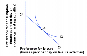
The diagram below illustrates the trade-off between allocating time between leisure activities and income generating activities. The straight line is the 24 hour constraint, since there are a total of 24 hours in a day, and this is the maximum amount of hour workers can spend working or resting. If multiple days are being considered the maximum number of hours that could be allocated towards leisure or work is 16 — given that a person sleeps 8 hours on average. The allocation decision is taken by looking and the time constraint and the indifference curve labeled IC, which indicates the combinations of leisure and work that will give the individual a specific level of utility. The point where the highest indifference curve is tangent to the constraint line shows how much time a person will spend working and resting. In the diagram that would be point A.

Continuing on the same line of thought, if the preference for consumption is measured by income, rather than hours of work, the diagram can be redrawn as to show a variety of other effects. In that case, the slope of the budget constraint becomes the effective wage rate and point A, the utility maximizing point, now reflects the equality between the wage rate and the marginal rate of substitution of leisure for income, which is the first derivative of the indifference curve at that point, or its slope. Since that marginal rate of substitution is also the ratio of the marginal utility of leisure (MUL) to the marginal utility of income (MUY), then:
Pic2
If real wages increases, this worker’s constraint line will pivot up from X,Y1 to X,Y2, showing that he can now purchase more goods and services by doing the same amount of work. Consequently, the worker’s utility will increase from point A on IC1 to point B on IC2. The shift from point A to point B can be explained by looking at the income and substitution effects.
Pic3
The shift in the above diagram can be shown in a different way, depicting both effects separately. The pure income effect is shown as the movement from point A to point C in the diagram below. Consequently, consumption increases from YA to YC and leisure time increases from XA to XC.
As the wage rate rises, the worker will also substitute work hours for leisure hours in order to take advantage of the higher wage rate, or substitute away from leisure because of its higher opportunity cost. That effect, the substitution effect, is represented by the shift from point C to point B. Pic4 The shift from point A to point B is the net result from both effects. The relative magnitude of the two effects depends on the circumstances. In some cases the substitution effect is greater than the income effect, whereas in other cases the income will be greater than the substitution effect. Pic5 Considering only the two effects, if the substitution effect dominates the income effect, the supply of labor curve will slope upwards and to the right, as it does at point E in the diagram below. This worker will choose to continue increasing the labor he supplies with the increasing wage rate up until point F where he is working HF hours. At that point, the income effect starts dominating and the worker will start reducing the amount of labor hours supplied. Where the supply curve is sloping upwards and to the right the elasticity of labor supply is positive and where it is sloping upwards and to the left it is negative (at point G). The direction of the slope is different for all individuals at the different levels of labor and income and in the next sections we will discuss why that is and what are the consequent results for the different workers.